Examples: from minimal to full

A code-first ladder through the forward pipeline. Each rung adds one step to the steps list and shows what it buys you - starting from sharp cells on black and ending at a full, noisy recording. Every step is optional and composable: a step that is absent simply contributes nothing (there is no hidden default-valued version running), so any rung below is a valid recording on its own and an honest control for the rung above it.

This is the static, copy-paste companion to the interactive anatomy notebook (which builds the same chain with live sliders). Every figure here is reproducible from the snippet beside it.

All rungs share one acquisition - a 200 µm field at 1.0 µm/px (8 µm sensor pitch ÷ 8× magnification), 20 s at 20 fps:

from minisim import Acquisition, Optics, ImageSensor

acq = Acquisition(
    fps=20.0,
    duration_s=20.0,
    optics=Optics(magnification=8.0),                  # 8x
    image_sensor=ImageSensor(
        n_px_height=200, n_px_width=200,
        pixel_pitch_um=8.0,                            # 8 / 8x = 1.0 µm/px -> 200 µm FOV
    ),
)

1. Minimal: cells on black

The smallest spec that produces a movie: place neurons, give them calcium activity, and composite them into pixels. No optics step, so the cells are sharp disks; no sensor, so the movie is clean continuous intensity.

from minisim import Spec, simulate, PlaceNeurons, CellActivity, Composite

rec = simulate(Spec(acquisition=acq, seed=1, steps=[
    PlaceNeurons(),     # where the cells are (3-D volume)
    CellActivity(),     # calcium traces so they blink
    Composite(),        # cells -> the movie
]))

composite and cell_activity are not optional “effects”: without traces, composite has nothing to scale the footprints by and the movie is blank. The recording already ships full ground truth - cell centers, the planted footprints A, and the clean traces C/spikes S:

gt = rec.ground_truth
gt.centers_um      # (n, 3) cell centers as (z, y, x) µm
gt.A_planted       # (n, H, W) sharp footprints
gt.C, gt.S         # (n, frames) calcium traces and spike counts

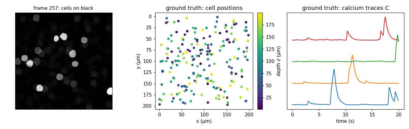
Left: a frame (cells on black). Middle/right: ground truth - cell positions colored by depth z, and a few calcium traces C.

2. Add optics: blur and dimming by depth

The optics step degrades each footprint by its depth: diffraction + defocus (distance from the focal plane) + scatter blur, plus scatter attenuation and the NA² collection loss. Cells away from the focal plane blur out; deep cells also dim.

from minisim import CellOptics

rec = simulate(Spec(acquisition=acq, seed=1, steps=[
    PlaceNeurons(), CellActivity(),
    CellOptics(),       # depth-dependent blur + dimming
    Composite(),
]))

CellOptics has no tunable fields - the blur and attenuation are fully determined by each cell’s depth and the physical Optics/Tissue constants on the acquisition. With focal_depth_in_tissue_um="auto" (the default) the focal plane is resolved here; the per-cell results land in ground truth:

gt = rec.ground_truth
gt.focal_depth_um                  # the resolved focal plane (µm)
gt.A_planted, gt.A_observed        # (n, H, W) sharp vs optically-degraded footprints
gt.observed_sigma_px, gt.depth_um  # (n,) per-cell blur width and depth
gt.in_focus                        # (n,) within the depth of field?

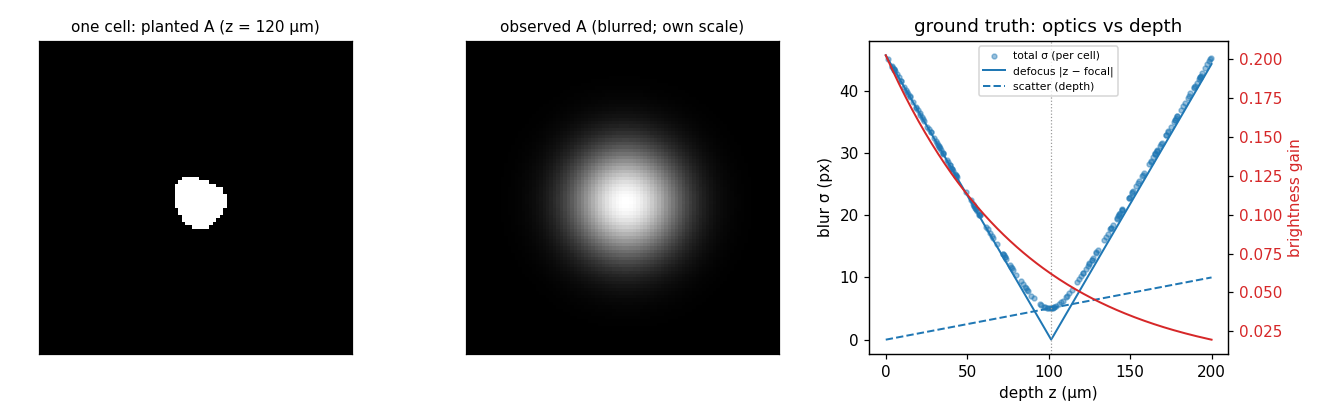
One cell from this recording, before and after optics: its planted footprint A (the sharp truth) and its observed footprint (blurred and dimmed), shown at its own scale to reveal the blur shape. Right: ground truth across the whole population - the per-cell total blur (dots) decomposed into defocus (the “V”, zero at the focal plane) and scatter (the ramp growing with depth), which add in quadrature, while brightness (red) falls with depth.

3. Add brain motion

brain_motion rigidly translates the tissue frame per frame and crops the sensor FOV from a margin-padded canvas (sized automatically), so real off-FOV tissue moves into view. This is the motion you would run motion-correction against.

from minisim import BrainMotion

rec = simulate(Spec(acquisition=acq, seed=1, steps=[
    PlaceNeurons(), CellActivity(), CellOptics(), Composite(),
    BrainMotion(),      # rigid (dy, dx) translation per frame
]))

gt = rec.ground_truth
gt.shifts            # (frames, 2) per-frame (dy, dx) displacement in PIXELS

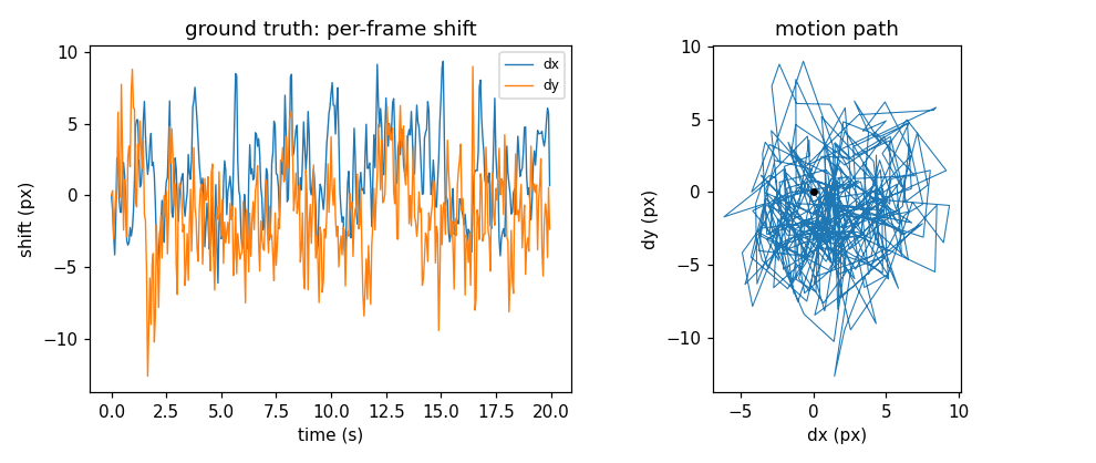
Ground truth: the per-frame (dy, dx) shift over time (left) and the 2-D motion path (right). The default "physical" model is a damped oscillator driven by a locomotion rhythm plus broadband sloshing - the exact displacements are recorded, so recovered shifts can be scored against them.

4. Add neuropil background

neuropil adds the diffuse haze from the surrounding dendritic/axonal felt: a smooth spatial field modulated by a biologically-driven temporal envelope (the local population’s lagged calcium plus an independent slow drift).

from minisim import Neuropil

rec = simulate(Spec(acquisition=acq, seed=1, steps=[
    PlaceNeurons(), CellActivity(), CellOptics(), Composite(),
    Neuropil(),         # additive diffuse background
]))

gt = rec.ground_truth
gt.neuropil_spatial      # (n_comp, H, W) smooth spatial components
gt.neuropil_temporal     # (n_comp, frames) per-component envelopes
gt.neuropil_population   # (frames,) the population activity driver

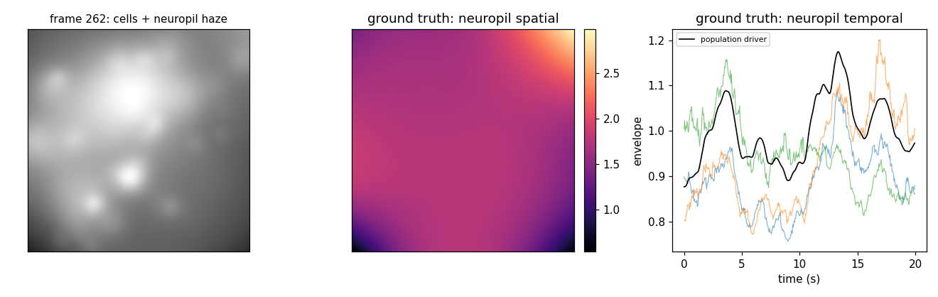
Left: a frame - cells (dimmed by optics) sitting in the diffuse haze. Middle/right: ground truth from this recording - the neuropil’s smooth spatial field (sum of its components) and the per-component temporal envelopes with the population driver (black). The haze tracks population activity rather than blinking, so it is contamination demixing must separate from the real traces.

5. Add vasculature: a static landmark and a confound

vasculature grows depth-resolved branching blood vessels and multiplies a dark transmission mask into the movie (vessels absorb both the excitation going in and the emission coming out). It is a tissue-domain step applied right after neuropil and before brain_motion, so the vessel pattern is fixed in the brain frame and rides the motion crop rigidly with the cells. That is exactly what makes it useful two ways: a temporally static, high-contrast landmark for motion-correction to register against (the cells flicker with activity, the vessels do not), and a tunable confound - a vessel crossing a soma absorbs its light and corrupts its footprint and trace.

It is off by default (enabled=False, empty layers); turn it on with at least one VesselLayer. Each layer is blurred by the defocus + scatter at its own depth_um, so a vessel near the focal plane is a crisp dark thread while one far from focus softens into a broad shadow (the same depth blur the cells get).

from minisim import Vasculature, VesselLayer

rec = simulate(Spec(acquisition=acq, seed=1, steps=[
    PlaceNeurons(), CellActivity(), CellOptics(), Composite(), Neuropil(),
    Vasculature(enabled=True, layers=[       # off by default; one layer here
        VesselLayer(depth_um=100.0, n_roots=4, root_radius_um=10.0, opacity=0.8),
    ]),
]))

The occlusion is scored, not hidden. The vessel mask is recorded, and each cell gets a footprint-weighted vessel-overlap fraction so you can stratify recall or footprint-correlation by vessel burden; a vessel over a soma also dims its peak in the detectable test. The footprints (A_observed) themselves stay vessel-free - they are the single-cell optical truth the confound is measured against:

gt = rec.ground_truth
gt.vasculature_mask           # (H, W) static vessel transmission in (0, 1]
gt.vessel_overlap_fraction    # (n,) per-cell occlusion: 0 = clear, ->1 = fully under a vessel
gt.detectable                 # (n,) now folds vessel transmission into the peak SNR test

List several VesselLayers to stack scales and depths (e.g. a shallow large-caliber layer above the cells plus a deeper fine-capillary bed).

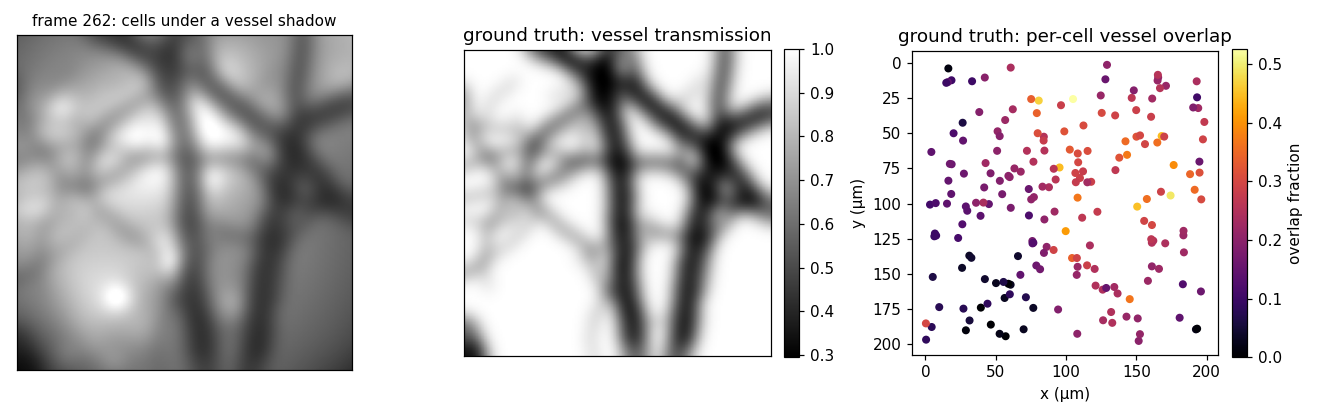
Left: a frame - cells and haze under a branching vessel shadow. Middle: ground truth - the static vessel transmission mask (vessels dark), sharp here because the layer sits near the focal plane. Right: ground truth - each cell colored by its vessel_overlap_fraction, the scoreable confound; cells under a vessel light up.

6. Add the static optical fields

Three scope-fixed fields, all smooth and static (they do not move with the brain): illumination_profile (excitation brighter at center), vignette (collection light loss toward the corners), and leakage (an additive stray-light glow). Each is recorded to ground truth as an (H, W) field.

from minisim import IlluminationProfile, Vignette, Leakage

rec = simulate(Spec(acquisition=acq, seed=1, steps=[
    PlaceNeurons(), CellActivity(), CellOptics(), Composite(), Neuropil(),
    IlluminationProfile(),   # excitation falloff (multiplicative)
    Vignette(),              # collection falloff (multiplicative)
    Leakage(),               # stray-light baseline (additive)
]))

gt = rec.ground_truth
gt.illumination, gt.vignette, gt.leakage    # (H, W) static fields

These three are exactly the smooth, static background that minian’s “glow removal” estimates and strips (the multiplicative falloffs and the additive leakage), because the cells are sharp and moving while the fields are not.

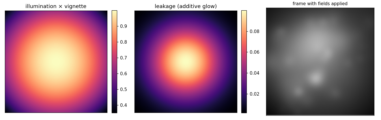
Left/middle: the combined illumination × vignette field and the additive leakage glow. Right: a frame with the fields applied - bright center, dim corners, plus the central haze.

7. Full recording: add the sensor

sensor is the last step and the only one that produces integer counts: it turns the clean intensity into raw 8-bit ADC counts via Poisson shot noise, Gaussian read noise, gain, and quantization. This is where SNR becomes real (it emerges from the photon budget against the noise floor, never set by hand) and where the detectable flag and the auto-focus yield go live.

from minisim import Bleaching, Sensor

rec = simulate(Spec(acquisition=acq, seed=1, steps=[
    PlaceNeurons(), CellActivity(),
    Bleaching(),             # cell-domain: slow activity-driven photobleaching
    CellOptics(), Composite(), Neuropil(),
    BrainMotion(),
    IlluminationProfile(), Vignette(), Leakage(),
    Sensor(),                # photons -> noisy integer counts
]))

gt = rec.ground_truth
gt.detectable        # (n,) cells whose transient clears the sensor noise floor
rec.observed         # (frames, H, W) raw 8-bit counts

Sensor.photons_per_unit is the exposure (the photon flux per intensity unit). It scales every light source in the frame equally - cells, neuropil, vasculature, leakage - and sets the shot-noise regime: raising it (or the sensor gain) brightens the recording, and a higher photon budget also lifts the shot-noise-limited SNR. It is a fixed number, not auto-leveled; make_recording() ships a well-chosen default so a fixture is bright and clear out of the box, and you pass an explicit Sensor(photons_per_unit=...) for a dimmer or brighter run.

(bleaching is cell-domain, so it sits before composite with the other per-cell steps. Its fade acts over minutes, so it is negligible in a 20 s clip - included here for completeness. vasculature is left out of this default chain because it is off by default and used deliberately as a confound (section 5); drop a Vasculature(...) step in right after Neuropil() when you want vessels.)

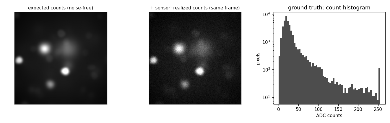
Left: the noise-free expected counts (the intensity the sensor sees, digitized without the random draws). Middle: the same frame with the sensor’s shot + read noise - identical scene, only the noise differs. Right: the count histogram; the spike at 255 is saturation clipping at the 8-bit ceiling.

Both panels come from the same run (until="leakage" for the left): with a sensor present, the optics "auto" focus switches to the yield-maximizing plane, so a separate sensorless run would focus on a different plane and show a different scene - the sensor is what makes the focus decision go live.

Writing a video, and two gotchas

Any rung can be written straight to a grayscale video (needs the notebook extra, pip install "minisim[notebook]"):

rec.write_video("recording.avi", vmax=float(rec.observed.max()))

• Without a sensor step you must pass vmax. A sensorless movie is continuous intensity with no ADC range, so there is no natural white point; write_video/simulate_video raise unless you give one. With a sensor, vmax defaults to the full ADC range automatically.

• Mind motion vs FOV. A spec warns (SpecWarning) if the motion extent exceeds ~5% of the FOV. At this 200 µm field the default ~10 µm motion is right at 5% (fine); on a smaller FOV, either lower BrainMotion(motion_amplitude_um=...) or widen the field with a coarser pixel.

For the same progression with live sliders and the physics narrated stage by stage, see the anatomy notebook.